Tukey (1977) and Mosteller and Tukey (1977) propose a simple rule for transforming non-linear relationships into linear using the ladder of powers.
The approach begins by determining the nature of curvature in the relationship. If a scatter-plot cannot reveal any obvious pattern then you can observe three sets of bivariate coordinates compare the two slopes, from the first to the second coordinate and from the second to the third coordinate. These points on the plane should be equidistant in the probability distribution, as for example the first quartile, the median and the third quartile, or the 5th percentile, the median and the 95th percentile. Avoid going too close to the tails if you suspect extreme values.
If the curvilinear relationship is monotonic (strictly increasing or strictly decreasing) then you can apply the ladder of powers to transform either the y variable or the x variable, or both. Sometimes it suffices to transform just one variable but exponential relationships usually require transformation of both variables.
Motivating application
Consider an abalone fishing business. Collecting wild abalone is a very difficult operation and can be dangerous. Abalone businesses need to give clear instructions to their divers to what to look for. Also, there are strict quotas on how many wild abalone can be collected, so when diving and faced with alternatives the diver needs clear instructions on which abalone to collect and which they should leave for the future.
In a more practical matter, when diving for abalone there is only that much you can do. In 10 meters depth, visibility is limited and it is impossible to judge weight. It is also impossible to judge shucked weight which is how prize is determined. The only useful information that the diver can use is either the length or the diameter of abalone, against a point of reference that the diver could carry.
Therefore, we want to know what is the relation between abalone length or diameter and the shucked weight. It is reasonable to say that the bigger the abalone shell the larger the animal would be residing in the shell.
First we compare the abalone diameter with the abalone length using a quantile-quantile plot: these are two potential predictors of abalone’s shucked weight. We find that their standardised distribution is virtually indistinguishable, thus it does not matter which one to use as predictor for shucked weight. This of course makes perfect sense as diameter is a direct function of length.
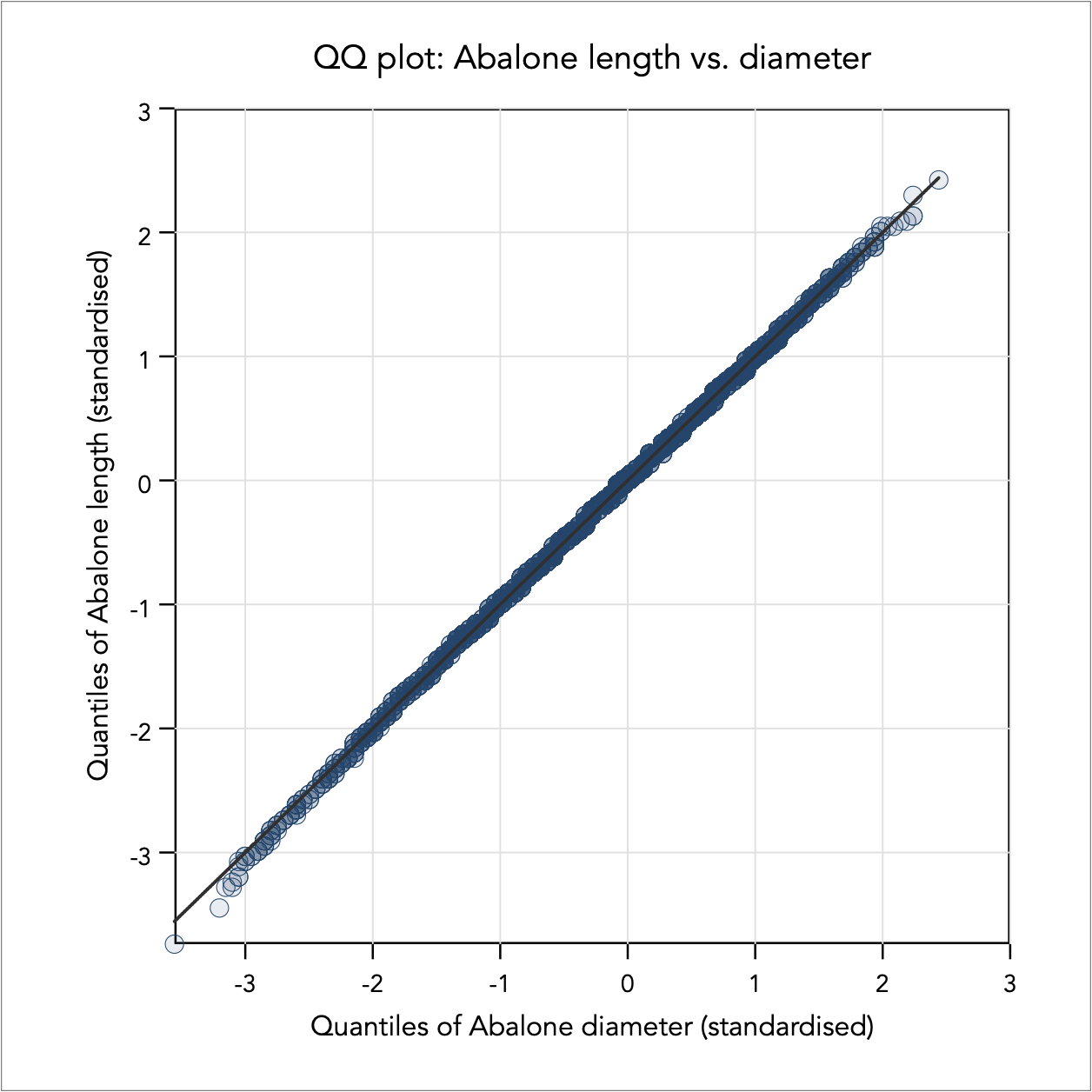
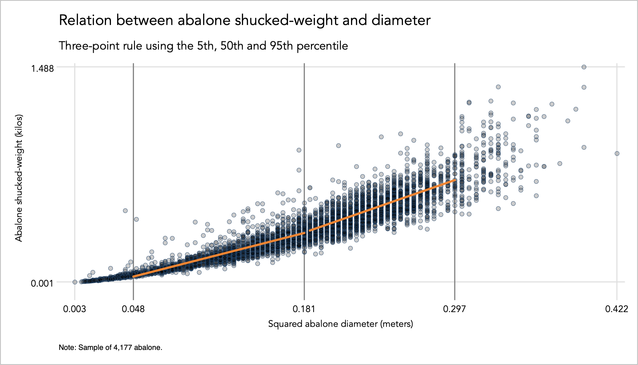
I choose to continue the analysis using diameter as it is easier to understand in the deep. Next, I visualise the relation between shucked weight and diameter:
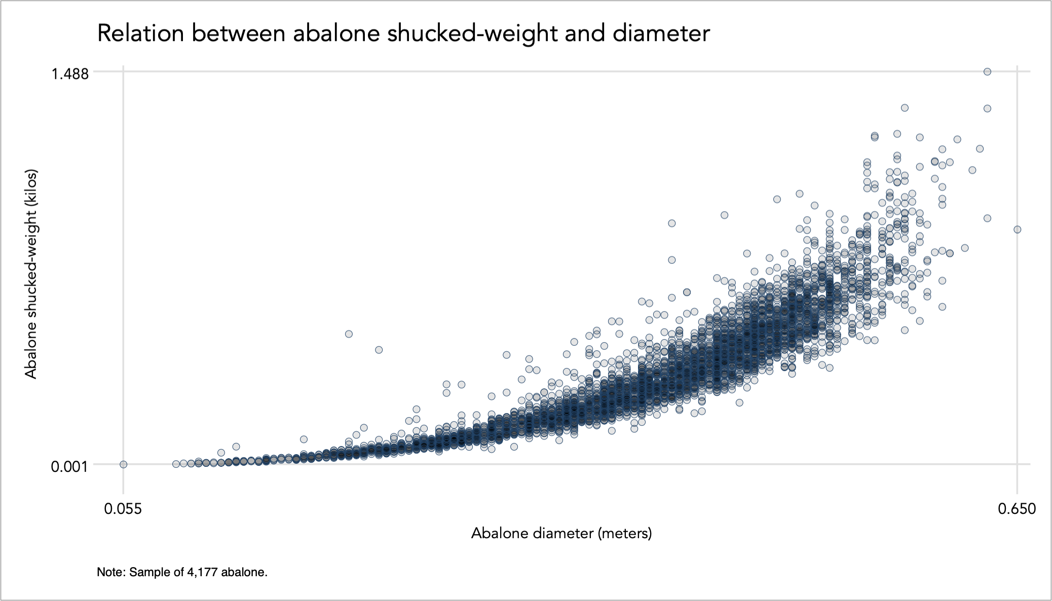
The relation between diameter and weight is strong but non-linear. Also notice how the variance increases as we move to larger values. To linearise the relation, we could go through the same process of individually assessing the need for transformation as demonstrated in Transformations for [0,+∞) variables, or we could consider the joint relation cohesively.
Three-point method
Tukey (1977) and Mosteller and Tukey (1977) propose a simple rule for transforming such non-linear relationships into linear using the ladder of power transformations. The approach begins by determining the nature of curvature in the relationship. To do so, we need to calculate three equidistant bivariate coordinates and compare the two resulting slopes. For example, let’s calculate ratio of the two slopes from the set of 35th percentiles to the 50th percentiles, and slope from the 50th percentiles to the 65th percentiles:

The ratio between the two slopes is equal to 1.36, hence indicating that the second slope is about 1.36 times steeper than the first slope. This information tells us that the relation is fairly linear in the middle of the distribution. Extending the range of the slopes to the first and third quartiles increases the ratio between the two slopes to 1.51. Extending the range of the slopes further to the 5th and 95th percentiles the ratio now becomes equal to 2.43 and the two slopes look like this:
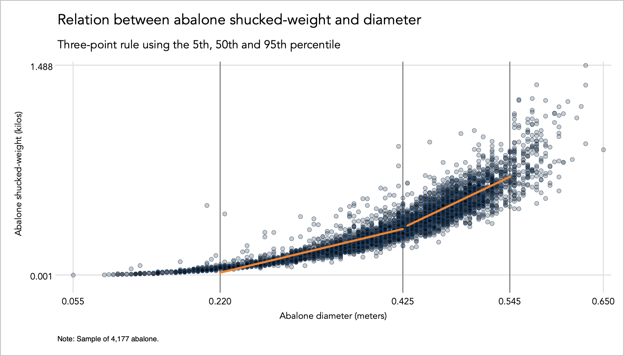
So we can conclude that the nonlinearity is more evident in the shoulders and the tails of the bivariate relation.
Bulging rule
There is evident need for linearisation. To guide the choice of appropriate transformations, Tukey (1977) and Mosteller and Tukey (1977) describe the following bulging rule (a heuristic method similar to the ladder of powers):
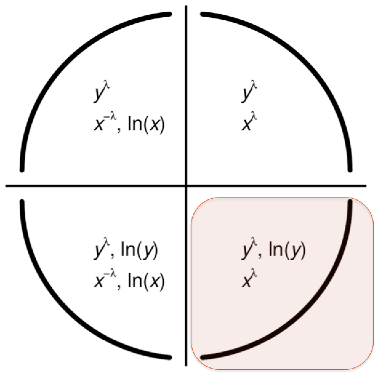
The relation between abalone diameter and shucked weight described above bulges similarly to the red highlighted area. In this case, the bulging rule suggests the use of a positive power transformation or log transformation on shucked weight, and a positive power transformation on the abalone diameter.
I start by searching for the right power transformation for abalone diameter, using Newton’s method as described in Transformations for [0,+∞) variables. The optimisation approach returns the power of 2.0526 for minimising skewness at -0.0000104. To ease interpretation, I round the power to 2 and apply this transformation that results in skewness -0.0265442, still fairly close to zero. I graph again the relation using the three-point method:
The ratio of the two slopes is 1.62, a considerable improvement from the earlier 2.43. Sometimes, taking the transformation of one variable suffices to linearise the relation, but not in this case. I repeat Newton’s method for the weight variable, which returns the power of 0.5766 that minimises skewness close to zero. Again, I choose to round this power to 0.5 given its intuitive interpretation as square root, and I can live with the slightly excessive skewness of -0.1413. The relation based on both transformation looks as follows:
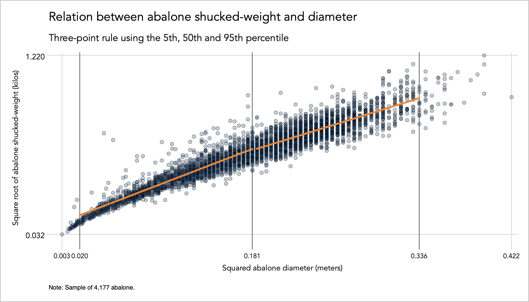
Note how the curve’s bulge has slightly switched, and the ratio of the two slopes is now less the one, and is equal to 0.9426. This is because I chose to round the optimal power transformations for diameter from 2.0526 to 2 and for weight from 0.5766 to 0.5, in order to ease interpretation of the relation. If we choose to apply the optimal powers then the relation would be a straight line.
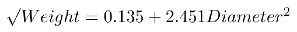
If we are happy with the result of the rounded power transformations of producing sufficient linearity then we can proceed to estimate an OLS relation, however with robust standard errors considering the evident heteroscedasticity in the errors, here due to the magnitude of the errors increasing as diameter becomes larger. The OLS regression returns the following estimates with an R-squared of 90.4%:
Business context
There is need to put this discovery in a business context. Experience divers can recognise with fair accuracy what is a small, medium size and large abalone, and we have found that the weight has a nonlinear relation with diameter, as described in the equation just above. The OLS estimates tell us that on average for every unit increase in the squared diameter of abalone will lead to 2.451 increase in the square root of weight. This is still a non-intuitive result that would be hard to communicate to divers, and the reference to average calculations is also not very helpful.
We need to translate this discovery into easy instructions to guide divers in what to look for. Considering that the price for abalone can go as high as $100 per kilo, making the right choice has great consequences.
Let’s define the following rules of thumb for the divers. Let’s label the abalone with diameter close to the 10th percentile as ‘very small’, the abalone with diameter close to the 30th percentile as ‘small’, and similarly for the following:
| Description | Percentile | Diameter | Weight (kilos) | Weight ($) |
| Very small | 10th | 0.265 | 0.094 | $9.4 |
| Small | 30th | 0.365 | 0.213 | $21.3 |
| Ordinary | 50th | 0.425 | 0.333 | $33.3 |
| Large | 70th | 0.470 | 0.457 | $45.7 |
| Very large | 90th | 0.525 | 0.657 | $65.7 |
where Weight (kilos) is calculated as follows:
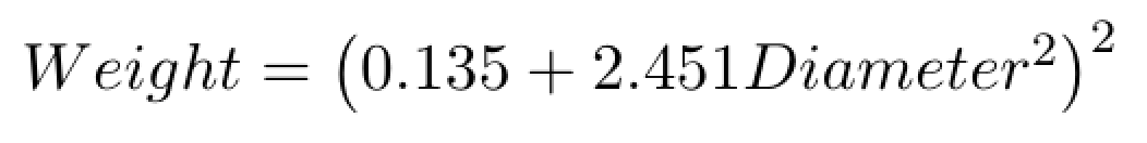
and Weight ($) is an approximation for sales revenue and is simply equal to Weight (kilos) times $100 (a rough price for shucked abalone per kilo). Notice how the revenue increases in a non-linear manner as diameter increases. Very small abalone return about $9.4 per shell, and going from Very small to Small increases revenue by 21.3-9.4=$11.9. However, the increase from Large to Very large return nearly double as much, at 65.7-45.7 = $20 more revenue.
That is to say, the shucked weight increases at an increasing rate as diameter becomes larger. In biological terms, this suggests that first the shell grows much faster than the animal itself to a certain extend (here shown at about the median diameter), and then the animal starts growing faster than the shell itself.
This brings us to a very important business insight. It pays off to leave Very Small to Ordinary sized abalone, and fish only Large to Very large abalone. To ensure that this is the case, we can provide divers with a non-corrosive abalone guide of what constitutes to be an Ordinary size, and collect only those that are larger. Focusing on the much large abalone not only ensures the maximisation of profit in selecting the right size but could also help control supply.
Back to [0,+∞) variables ⟵ ⟶ Continue to (–∞,+∞) variables
