As explained in the discussion of points-to-lines-to-areas, line visual implantations are constructed by connecting points on a coordinate plane.
The software default for connecting points is direct connection, that is to say drawing a direct line between the successive coordinate points (i.e. the shortest distance between two points). However, depending on the data properties it may be necessary to switch to a stairstep or stepstair line connection.
To demonstrate the difference between connecting styles, here is how it would a set of coordinates would look when connected using the three different approaches. These coordinates are (y, x) = (1, 1), (1, 2), (1.5, 3), (0.5, 4), (0.5, 5):

Direct connection
The direct connection is suitable in encoding the angle between two points in the coordinate plane. For example, it is appropriate for encoding the rates of change in stochastic time-series data containing regular random variation.
In the illustration just above, the progression from the first coordinate point at (1, 1) to the next at (1, 2), indicates no change (the line is flat). The progression from the second point at (1, 2) to the third at (1.5, 3) indicates an increase at the rate of (1.5 – 1)/1 = 0.5 or 50%, and the slope between the two points can be calculated as follows:

Similarly, the progression from the third point to the fourth has slope -1, or 45 degrees angle. To understand the ramifications of correctly encoding angles, see the discussion
I demonstrate such examples in the analysis of Taiji Cove drive hunt, Labour equality and human development, US life expectancy of males, US federal tax revenue, Market value function, and more. In all these examples, a common feature is that the the time-series data regularly fluctuates from one time step.
Step functions
The stairstep and stepstair connections are suitable to representing step functions. A step function describes a piecewise constant function within successive disjoined intervals and can be represented as follows:
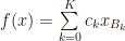
where k = 0,1,…,K is the number of step intervals, ck is a constant specific to each interval, and Bk is the specification of the kth interval that is a function of range in x.
The difference between stepstair and stairstep is in the specification of range in each Bk interval, that may include or exclude the endpoint of each interval.
Using the example dataset presented above, the stepstair function can be written as follows:
![f(x)= 1x_{[1,2]} + 1.5x_{(2,3]} + 0.5x_{(3,4]} + 0.5x_{(4,5]}](https://s0.wp.com/latex.php?latex=f%28x%29%3D+1x_%7B%5B1%2C2%5D%7D+%2B+1.5x_%7B%282%2C3%5D%7D+%2B+0.5x_%7B%283%2C4%5D%7D+%2B+0.5x_%7B%284%2C5%5D%7D+&bg=ffffff&fg=1e0d03&s=0&c=20201002)
The key notation here is the use of parenthesis or squared brackets in specifying range. A parenthesis indicates exclusion of that value, where a squared bracket indicates inclusion of that value. For instance, 0.5x(3,4] indicates that f(x) = 0.5 from x greater than 1 and up to the value of 2 inclusive.
The respective representation for the stairstep function is:
![f(x)= 1x_{[1,2)} + 1.5x_{[2,3)} + 0.5x_{[3,4)} + 0.5x_{[4,5]}](https://s0.wp.com/latex.php?latex=f%28x%29%3D+1x_%7B%5B1%2C2%29%7D+%2B+1.5x_%7B%5B2%2C3%29%7D+%2B+0.5x_%7B%5B3%2C4%29%7D+%2B+0.5x_%7B%5B4%2C5%5D%7D+&bg=ffffff&fg=1e0d03&s=0&c=20201002)
Stepstair line connection
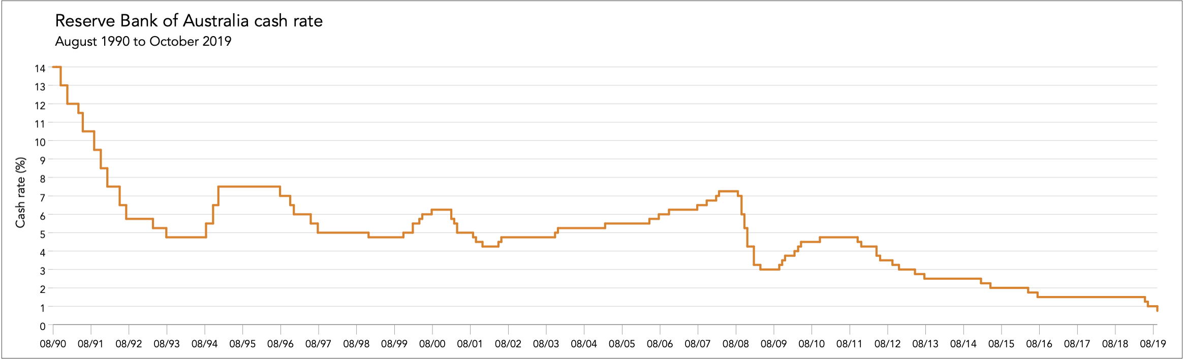
Stepstair functions change value at the beginning of each successive interval. As an example, consider encoding the evolution in cash rates.
Reserve banks (aka central banks) around the world have the task of regulating monetary policy by setting cash rates (federal funds rates in the US). Rates can change in distinct points in time following monthly meetings in reserve banks, but rates do not change every month. It is often the case that once a rate changes, it would a some months before the rate changes again. In another words, the rates will remain fixed during a time period interval, i.e. the evolution function of rates follows a step function.
For example, the Reserve Bank of Australia set the cash rate to 1.5% as at 3 August 2016, which stayed at the level until 8 May 2019 where it changed to 1.25% that took effect immediately. This means that the cash rates follow a stepstair function, which can be written as follows:

This representation means that the rate of 1.5% took effect as at 3 August 2016 up to but excluding 8 May 2019, at which point the rate changed. Thus, the most appropriate form of visualisation of the timeline evolution of cash rates is the stepstair connection, as follows:
Stairstep line connection
Stairstep functions change value at the end of each successive interval. I demonstrate an application in the analysis of capital stock-and-flow, which is concerned with the analysis of stocks and flows as observed from the accounting data generating process.
Specifically, given the opening stock as observed from the Statement of Financial Position, the addition of flows as reported in the Statement of Cash Flows and the Income Statement give the closing stock. This underlying structure of the data properties requires the use of a stairstep line connection.
Specifically, the question of visually encoding capital stock-and-flow can be represented in the following form, as a stairstep function:
![\textnormal{K}_{[t,t+1)} + \textnormal{CPX}_{[t,t+1)} - \textnormal{DEP}_{[t,t+1)} - \textnormal{DIS}_{[t,t+1)} + \textnormal{OTH}_{[t,t+1)} = \textnormal{K}_{[t+1,t+2]}](https://s0.wp.com/latex.php?latex=%5Ctextnormal%7BK%7D_%7B%5Bt%2Ct%2B1%29%7D+%2B+%5Ctextnormal%7BCPX%7D_%7B%5Bt%2Ct%2B1%29%7D+-++%5Ctextnormal%7BDEP%7D_%7B%5Bt%2Ct%2B1%29%7D+-+%5Ctextnormal%7BDIS%7D_%7B%5Bt%2Ct%2B1%29%7D+%2B+%5Ctextnormal%7BOTH%7D_%7B%5Bt%2Ct%2B1%29%7D+%3D+%5Ctextnormal%7BK%7D_%7B%5Bt%2B1%2Ct%2B2%5D%7D&bg=ffffff&fg=1e0d03&s=0&c=20201002)
where K is capital investment, CPX is capital expenditure, DEP is depreciation, DIS is disposals, and OTH are other relevant events such as impairments, revaluations and accounting adjustments.
Back to Multiple axes ⟵ ⟶ Continue to Reference lines
