Completeness requires that all relevant data is graphed. No cherry-picking is allowed. If there are any exclusions or censored values, these must be clearly identified as part the graph, perhaps in a note to the graph.
Completeness also concerns with providing all relevant information for decoding a graph, through external and internal identification, including axes scales, false origins, units of measurement, reference lines and functional forms.
Completeness in identification should not be sacrificed for maximising the data-ink ratio but must be achieved with reduced visual prominence. Readability is an important property of completeness that eliminates uncertainty about representation. If encoding is implicit, then the internal graph identification must be comprehensive and eliminate ambiguity.
For example, the graph on US abortions and cancer screenings discussed in the quality of decoding accuracy, is not only inaccurate but also incomplete, because it does not show the year-by-year data so we have no way of knowing how good are these linear projections. This graph is also incomplete in its lack of accountability, as it does not cite any data source (also the accompanying article does not cite thee data). In fact, after recovering the data from the Centers for Disease Control and Prevention, I discover that some of data used in that graph has been in fact fabricated.
Perhaps the most infamous example of incompleteness is the graph presented to the NASA’s executives on the relation between O-ring strength in the fuel rockets and temperature, on the eve of the Challenger’s launch. The lack of completeness in that graph led to catastrophic decision making.
The original report presented by Norton Thiokol was the following:
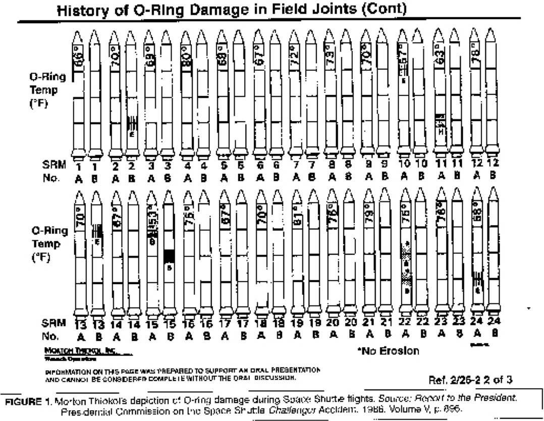
This graph is complete in the sense that it reports all data on all tests done on the pairs of rockets in different temperatures. However, this graph suffers from low relevance as it plagued with chart-junk that makes decoding nearly impossible. So, someone from NASA took the Norton-Thiokol graph and turned it into this scatter graph:
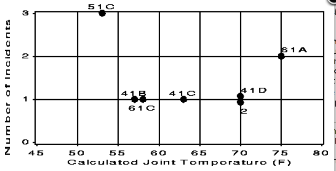
This scatter graph is now incomplete because it cherry-picks only the data from the tests that have recorded O-ring failures. It ignores all other data from the tests that were successful (i.e. with no failures). As a result, the message of this graph is that it is inconclusive to say whether there is a pattern between temperature and O-ring failure.
A complete graph would all the data, and perhaps even fit a predictive model of some sort, given that on the day of the launch the temperature was predicted to be between 26-29 degrees Fahrenheit (-3 degrees Celcius):
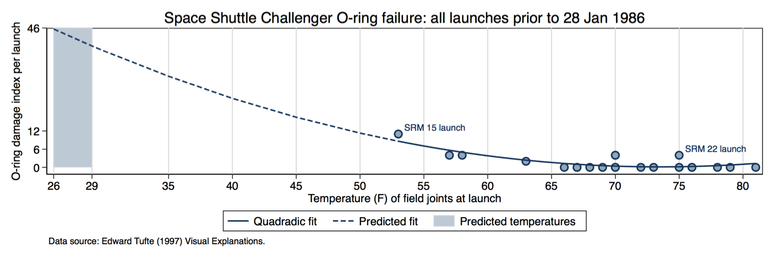
This complete graph makes it clear that there would be a certain certain failure if they launched the Challenger, which they did and the O-rings failed as predicted.
Always show the data
A data graph is never complete unless you actually show the data itself. Otherwise, we cannot conclude with confidence whether the data supports the analysis.
This point is best elucidated by the famous Anscombe (1973) quartet problem. Consider the following dataset that describes relations between pairs of variables (y1,x1), (y2,x2), (y3,x3) and (y4,x4):
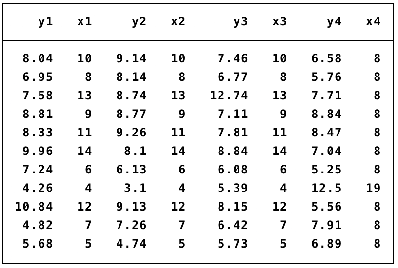
There is not much one can say by just looking at a table of data. What if I tell you that the mean and the standard deviation of every x variable is the same up to the sixth decimal point, and that the mean and the standard deviation of every y variable is the same up to the second decimal point. What if I also told you that the correlation between all pairs is the same at 0.816, and to convince you I will also show you the linear regression fit. Does this information on statistical estimates help you understand the bivariate relations?
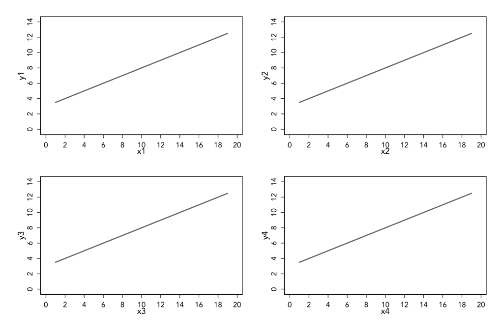
The above graph shows four predictive models that are fitted on the data, but we have no idea of knowing how good are these models because we cannot see the data! Hence, this graph is incomplete because we do not know if the data supports the model.
Here are the same linear predictive models with the data. For the top-left hand side relation of (y1,x1) the linear model fits quite well, but for the rest of the relations, the linear models are a complete nonsense.

Completeness as a second consideration
Remember that the first and foremost quality of data graphs is decoding accuracy. Completeness only comes second. That is to say, we can sacrifice completeness in order to satisfy accuracy. But if we do choose to violate completeness, then we must say so.
The scatter plots below show the relation of abalone height with their diameter from a sample of 4,177 abalone. Naturally, as the height of this marine mollusc increases the diameter should increase as well. The left-hand side graph suggests a very steep relation, probably in the order of 4-5 times increase of diameter for every unit increase in height. Notice that the steepness of the scatter plot relation suggests about 75-78 degrees angle, and this is equivalent to about a slope coefficient of about 4 to 5.
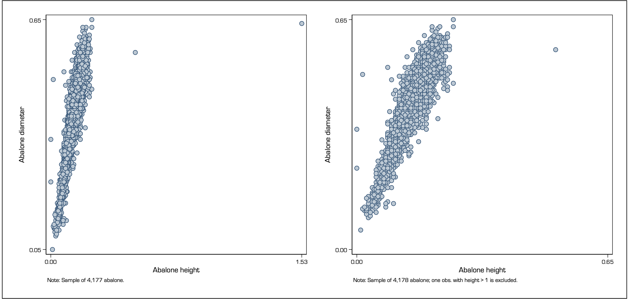
The left-hand-side graph has low decoding accuracy, because of the effect from one extreme value with height 1.53 and diameter 0.65. There are two ways to fix this inaccuracy: either extend the scale of both y-axis and x-axis to a common range from 0 to 1.53 given the same unit of measurement, or remove the extreme value. In this case, I prefer to do the latter because this extreme value appears to be an isolate case that is truly extraordinary. As a result, the right-hand side graph now suggests a slope of about 2.3 which equivalent to about 65 degrees angle.
This is a now a more accurate data graph but it is also incomplete. To compensate, I make sure to report in a note to the right-hand side graph of the exclusion of this one observation.
Back to Decoding accuracy ⟵ ⟶ Continue to Encoding relevance
