Nature and man produces positively distributed measures with range [0,+∞), e.g. the girth of a tree, the length of a river, height of a person, sales revenue, prices. The hard bound of zero produces highly skewed distributions that are difficult to analyse and especially visualise without a suitable transformation.
There are two approaches to transformation for reducing skewness. The heuristic approach is guided by prior knowledge and rules of thumb, and judges the appropriateness of transformation by looking at the resulting shape of the distribution, or by testing for symmetry and even normality. The alternative is the optimisation approach that calculates the degree of power transformation by minimising the objective function of zero skewness. The trade-off between the two is that the heuristic approach gives more intuitive results but the optimisation approach is more statistically accurate.
Tukey’s ladder of powers
Tukey (1957) explains how the distribution of [0,+∞) variables can be transformed to near symmetry using power transformations. Specifically, positively skewed data can be symmetrically transformed using negative powers, and negatively skewed data can be symmetrically transformed using positive powers. The greater the skewness the larger the absolute degree of power required to compress the sparse values and spread out the condensed part of the density. Tukey (1957) calls this rule the ladder of powers, that can be summarised in the following table:
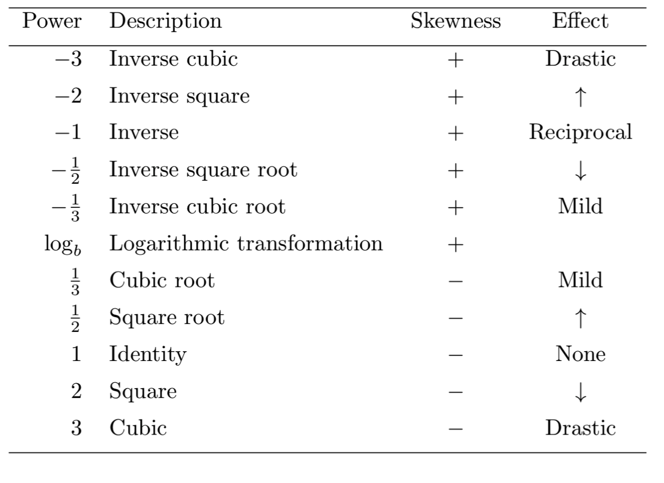
The ladder is not complete and may extend to higher or lower order powers. The power of zero does not belong to the ladder of powers because it is a degenerate distribution, i.e. y0=1 . However, Tukey explains that the log-transformation can take the position of the 0th power because its effect lies between the negative and positive powers.
The ladder of powers is a heuristic approach and the choice of powers as presented above is straightforwardly interpreted. However, going from the second to the third power translates into a huge transformative leap, and often the power that satisfies the criterion of symmetry requires a fractional power.
Optimisation approach
If sufficient symmetry cannot be found using the ladder of powers, then instead we could solve a simple optimisation functions for finding the fractional power that sets the objective function of skewness to zero. This can be easily done using Newton’s method (or Newton-Raphson method) that be implemented with Stata’s optimize command (or Microsoft Excel Goal Seek function). The do-file at the end of this page contains an example on how to employ the optimize command for this purpose.
Box-Cox transformations
The Box and Cox (1964) transformations are based on the optimisation idea of setting zero skewness by finding the suitable power λ and scalar c from the following objective function:
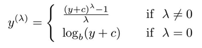
The Box and Cox (1964) family of transformations provides a more accurate objective function than just finding a fractional power in the ladder of powers. We can use again Stata’s optimize command to set up this objective function or just employ the ready-made command bcskew0.
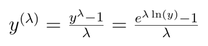
the added benefit of making it clear that the log-transformation takes the place of the power of zero. This key result can be demonstrated by rewriting the Box-Cox transformation as:
And using Taylor series expansion, we can show that:
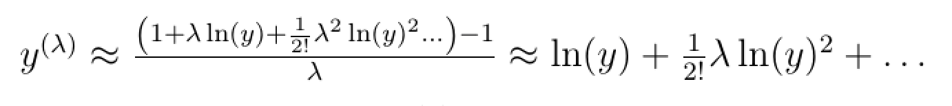
This means that as λ goes to infinity then y(λ) becomes equal to ln(y).
Logarithms
The logarithmic function is perhaps the most common and most powerful transformation for positively distributed ratio scale variables. The distance between two numbers on the logarithmic scale is equal to the distance of the base to the power of the two numbers on the nominal scale. For example, the change between 1 and 2 on the log10(x) scale is equidistant to the change of 101 and 102 in the nominal scale. Similarly, the change between 1 and 2 on the loge(x) scale is equidistant to the change of e1 and e2 in the nominal scale, where e ≈ 2.71828 is Euler’s number and loge(x) is also known as the natural logarithm, ln(x).
Log-transformations dramatically reduce scale through a monotonic transformation, that is by preserving the same distance between two values as in the nominal scale. Logs also have intuitive interpretation, e.g. log10(x) measures percentage change, log2(x) measures the doubling rate, log4(x) measures the quadrupling rate.
The log transformation is undefined for 0 hence the need to add the value of 1 to preserve the values of zero, e.g. for x=0 then log10(x+1) = 0. Logs return negative values for 0 < x < 1. In this respect, for interpretation it helps to remember the relation log(x)=−log(1/x).
Another important advantage of log-transformations is that if variable x follows the log-normal distribution then its natural log, ln(x), follows the normal distribution. This is a very convenient result because many naturally occurring magnitudes and economic measures closely follow the log-normal distribution.
Log-transformations also help linearise multiplicative relations. An example of this property is offered in the analysis of Greenhouse gas emissions per capita. As another example consider the power-sizing model that is sometimes used for obtaining an idea of the cost estimates of new industrial plants and equipment relative to the cost of existing comparable projects. The power sizing model is a multiplicative relation that is described as follows:
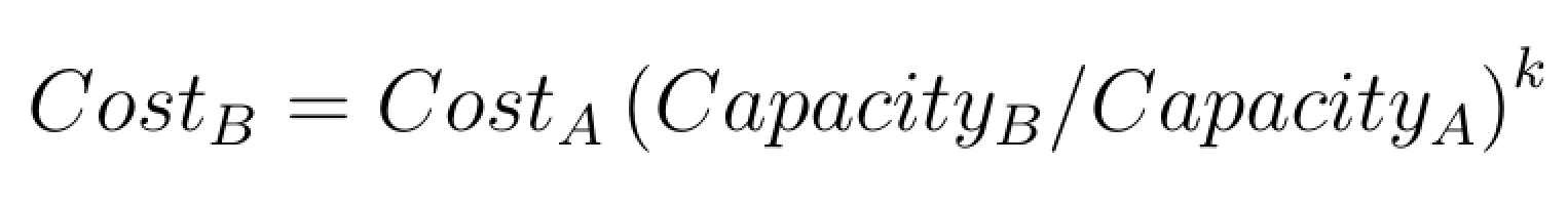
Taking logs linearises the relation and simplifies interpretation:

Application
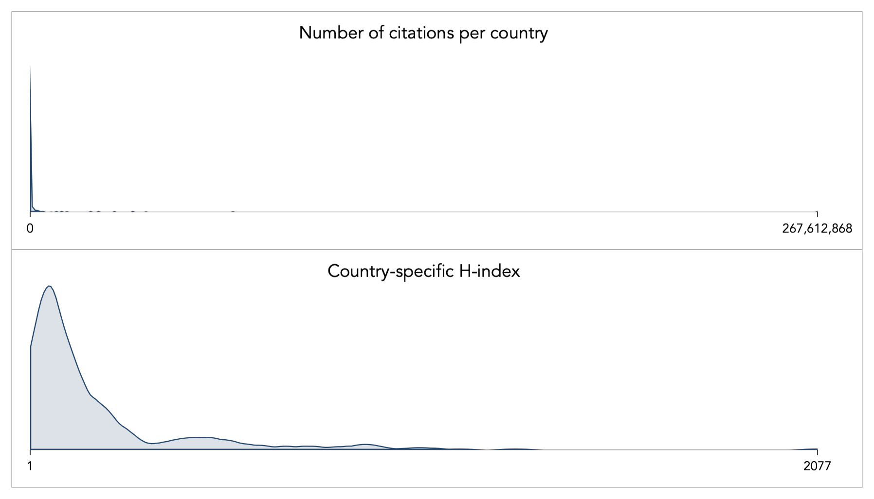
As an example of transformations for [0,+∞) variables, consider the relation between citations per country and the H-index (a type of impact factor for published original research). The dataset is sourced from www.scimago.com. The skewness for the number of citations is 11.66 and a for the H-index is 3.23; the kurtosis is 158.16 and 17.45 respectively. The shape of the distributions looks like this:
Let say, that we are interested in understanding how the number of scientific citations determine the H-index at the level of country. This relation using nominal values looks as follows:
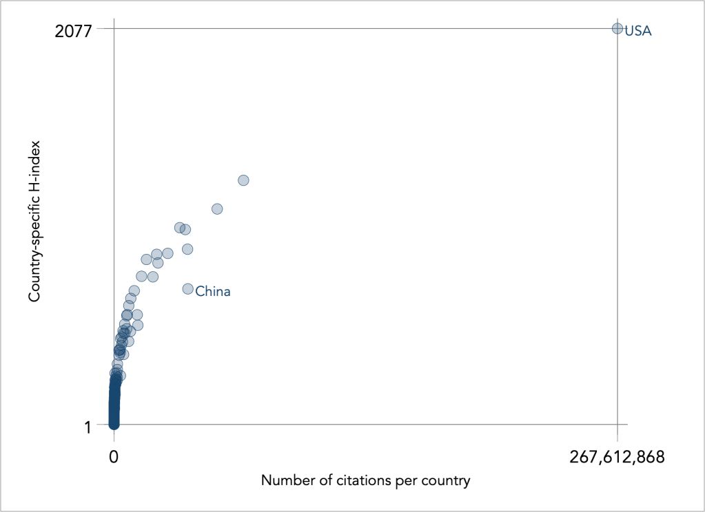
The relation is exponential, increasing at a decreasing rate, and is reflective of the high degree of skewness in the data. To alleviate the degree of positive skewness, Tukey’s heuristic ladder of powers prescribes the use of the log-transformation or negative powers. I try a collection of these powers:
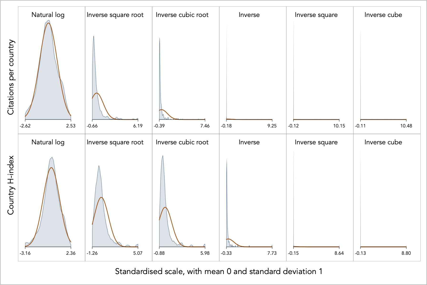
The superimposed orange line indicates the theoretical normal, following the standardisation of the variables. The log transformation for the citations per country appears to be spot on in turning the distribution into near Normal, whereas the rest of the transformations fail to produce a useful result. After all, only one transformation can succeed.
The log transformation for the country H-index is also the most successful but it does not appear to be an optimal result. In fact, the log transformation returns negative skewness, thus suggesting an excessive degree of transformation. In other words, from this result we can say that the appropriate degree of power transformation lies somewhere between 0 and 1, and not too close to the zero power.
We can also formally check the normality assumption using statistical tests. My favourite one is the Shapiro and Francia (1972, Journal of the American Statistical Association) test. Every statistical software should have this or some other similar test available. Here is the output from Stata’s sfrancia command:
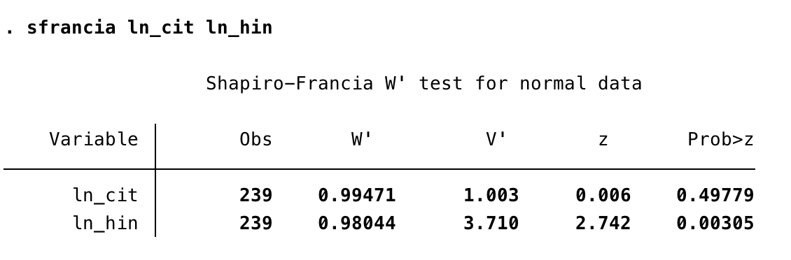
We cannot reject the hypothesis that the log-transformation of citations is normally distributed (variable ln_cit), but we reject the hypothesis for the log of country H-index (variable ln_hin).
We can also employ visual diagnostics to observe how close the data approximates normality, in addition to superimposing the normal curve on the kernel density function estimation as shown above. For example, we can look at how close the quantiles of the observed measurement are to the quantiles of the theoretical normal distribution (command qnorm), and how well the transformation fares against the standardised normal probability plot (command pnorm):
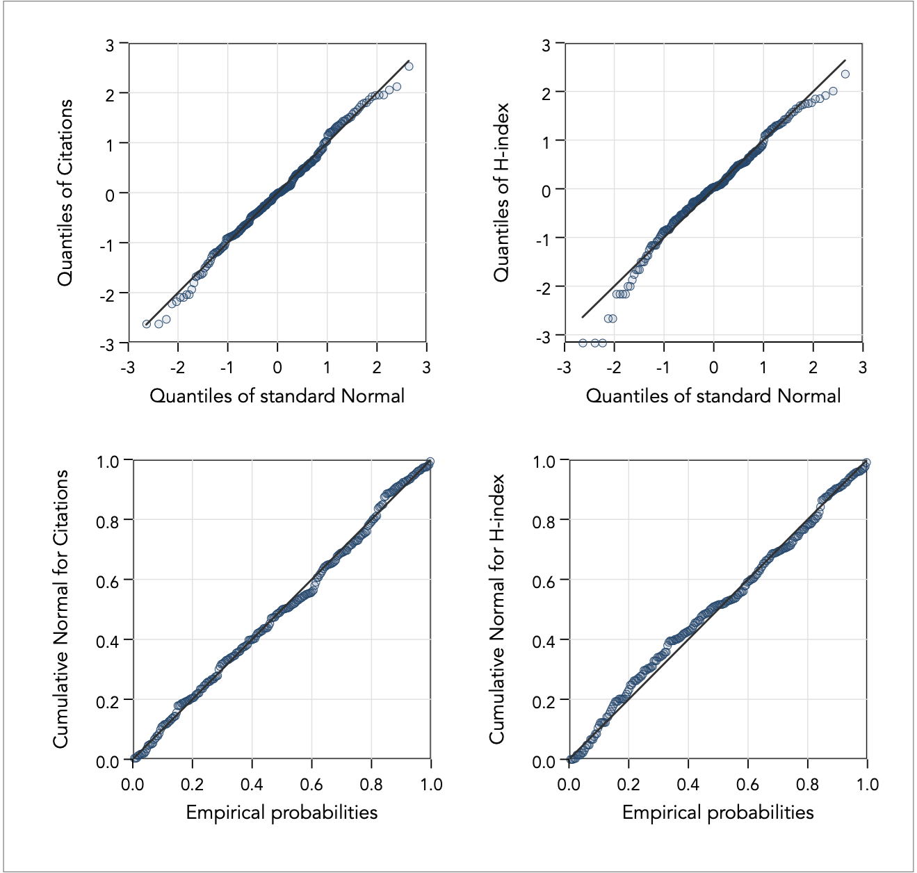
From the diagnostic plots we see that the problem of non-normality lies in the extremes of the distribution of the log-transformed H-index variable. Heuristics can get us this far, and often are good enough. We could stop here if we are satisfied and not too concerned about the limitations of the heuristic approach, or we could proceed to try and do better using the optimisation method.
Given the search for a suitable power in reducing skewness in the data, then we could search for the fractional power that minimises skewness. In the do-file provided at the end of this page, I demonstrate how to find this fractional power in two ways. First, using iterative substitution search until reasonable convergence given a tolerance limit for how close we want to get to zero skewness (I choose the fourth decimal point). This returns a fractional power of 0.1015 with skewness -0.0002902. Second, using Newton’s method and the optimize command, which returns the fractional power of 0.10155460 with skewness -0.0000515.
From this exploratory data analysis, we discover the following near-linear relation between country citations and country H-index:
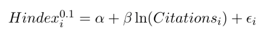
To ease interpretation of the relation I truncate the power of 0.1015 to 0.1. The relation is now additive and we can also estimate a simple OLS regression model which looks pretty convincing, as follows:
The OLS linear regression gives the following estimates:
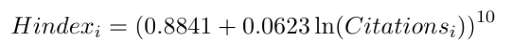
or equivalently:
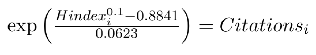
A policy maker can now say that an increase of citations by 1,000,000 would increase the H-index by 261.5. A Chinese policy maker could say that in order for China, with H-index 712, to reach the USA’s impact, with H index 2077, would need to attract another 153,292,942 citations from its published research (based on the increment of 2077 – 712=1365).
A more formal approach would be to apply the Box-Cox transformation as described above. We could solve that problem using Newton’s method. Stata’s bcskew0 command returns the power of λ=0.0071 for citations and λ=0.1015 for H-index, and this is a comforting result that corroborates the chosen transformations (remember that the power of near 0 has the effect of the log transformation).
To transform or not to transform?
A fundamental step in EDA is the transformation of variation into a more manageable and understandable form for analysis. Transformations aim to induce symmetry and contained variance, plus the added benefit of linearity and additivity that may follow when analysing relations. The ultimate prize is normality. Common transformations such as ratios, the logarithm, the inverse are easily interpretable. Other transformations may be difficult to explain. For example, how does one explain a x0.72 transformation ? But forgoing transformations means more complex modelling. An exponential relationship can be modelled using polynomials and an asymmetrically proportional relationship can be modelled as a 5-parameter logistic curve. Thus, you can trade convenience for complexity, but complicated parametric models must also be explained and justified accordingly, probably more so than transformations.
Back to Assessing normality ⟵ ⟶ To Linearising variables
