Assessing normality

Often, I see cases of using the kernel density estimator or even the histogram in evaluating how well the shape of a distribution fits a theoretical normal density. This is a mistake. The visual density estimators cannot help with this task.

There are two ways to visually assess normality: the probability-normal plot and the quantile-normal plot. These are described below.

Quantile-Normal plot

The rationale of Quantile-Normal plot (QN-plot) is the same as that of Quantile-Quantile plot (QQ-plot) discussed in the analysis of judging distributional form.

The QN-plot compares the quantiles of an observed distribution against the quantiles of the theoretical inverse normal distribution. This method is also known as probit plotting, a term coined by Rupert Miller (1997) in Beyond ANOVA: Basics of applied statistics.

A variable is approximately normally distributed if the i^th ordered value of x, denoted as x_(i), is close to the respective position of the inverse normal, where i = 1,2,…,n:

$\left(x_{(i)} - \mu_x\right) / \sigma_x \approx \Phi^{-1}\left[i/ n+1\right]$

The Stata reference manual [R] p.530 quotes Miller in giving the following advice: “If a deviation from normality cannot be spotted by eye on probit paper, it is not worth worrying about. I never use the Kolmogorov–Smirnov test (or one of its cousins) or the chi-squared test as a preliminary test of normality. They do not tell you how the sample is differing from normality, and I have a feeling they are more likely to detect irregularities in the middle of the distribution than in the tails” (Miller 1997, 13–14).

Consider a random sample of the 1,223 babies birthweight (in ounces) and their mothers’ gestation period (in days). This is the same dataset used in the analysis of judging distributional form. The QN-plots of birthweight and gestation are as follows:

Birthweight seem to follow closely the normal distribution with the exception of some deviation in the tails and especially the left-hand tail, but the distribution of gestation is evidently non-normal with much longer tail in the left and much shorter tail in the right.

It is worth noting that the Shapiro and Francia (1972) test for normality is based on the idea of the QN-plot, and is known to have the strongest statistical power (but become sensitive in large samples). In Stata, the Shapiro-Francia test is implemented with command sfrancia.

Normal Probability plot

The Normal Probability plot (NP-plot) is another visual guide, similar to the QN-plot, for assessing whether a sample is approximately normally distributed. A variable is approximately normally distributed if the following equation holds:

$\Phi \left[ \left( x_i - \mu_x \right) / \sigma_x \right] \approx i / \left(n+1\right)$

The NP-plot has a bounder range of variation from zero to one and begins and ends from a common set of points, the value of zero and the value of one. Thus, it is not able to tell much about tail behaviour as in QN-plot, but it is an excellent visual diagnostic for understanding distributional behaviour in the centre of the distribution:

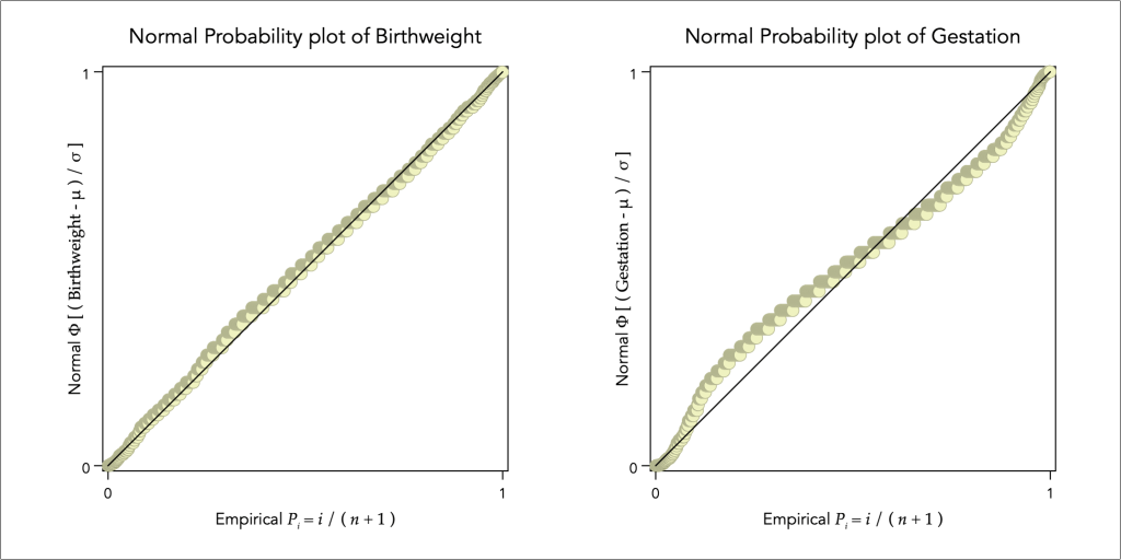
The NP-plot confirms that the birthweight distribution is not far from a normal distribution, but there is considerable deviations from normality for the distribution of gestation with negative skewness and high degree of kurtosis.

Probabilistic statements

Once we know how a variable is distributed we can make exact probability statements for answering two types of questions:

Q1: What is the probability p of a value X being less or greater than another value x? This question is answered using the cumulative density function.
Q2: Which values of x on the distribution are less or greater than a specified probability p? This question is answered using the inverse of probability function.

The Normal distribution requires knowledge of two parameters, the mean and standard deviation. For the random sample of the 1,223 babies, the mean birthweight is 119.62 ounces and the standard deviation is equal to 18.24, so we denote the distribution of birthweight as follows:

$Birthweight \sim N\left(119.62,18.24\right)$

An example of Q1 would be: “What proportion of babies will be born over 150 ounces (4.25 kilograms)?” As it is easier to work with the standard normal distribution, the cut-off value of 150 ounces is standardised to the score:

$z = \frac{150 - 119.62}{18.24} = 1.6656$

Then, we can use the cumulative standard normal distribution to answer this question, which is equal to 0.0479 or 4.79% of babies.

An example of Q2 would be: “Which birthweight is exceeded by the larger 1% of observations?” To answer this question first invert the standardised value in order to find the cut-off value, as follows:

$x = 18.24 \times z_{0.99} + 119.62$

where z_0.99 is the value of the inverse cumulative standard normal at the 0.99 probability, which is equal to 2.3263. Hence, the answer is:

$x= \exp\left(18.24\times 2.3263 + 119.62\right) = 162.05$

The answer explains that the birthweight exceeded by the larger 1% observations is greater than 162.05 ounces (4.59 kilograms).

Empirical Rule

Distribution analysis is all about understanding probabilities. We can work with a wide arrange of probability distributions, but many of these would be hard to explain to most.

`Yet, nearly every educated person understands the concept of the normal distribution, or the so-called ‘bell-shaped curve’, and the premise of the Empirical Rule that explains how much density lies around the mean within 1, 2, 3 or 4 standard deviations:

For a more generic ’empirical rule’ that can describe a wide range of distributions, see Chebyshev’s inequality.

The ultimate prize in Exploratory Data Analysis is indeed to find a way to transform variables into near normality, and such strategies are discussed in Transformations for [0,+∞) variables, Transformations for (–∞,+∞) variables, and Transformations for [0,1] variables.

Once we have a normal distributions, then we can work additively and understand relations much easier, because remember that for two independent random variables x and y:

$x\sim N\left(\mu_x,\sigma^2_x\right) \quad \textnormal{and} \quad y\sim N\left(\mu_y,\sigma^2_y\right)$