A ratio is a quantity that expresses two measurements relative to each other. Usually we think about a ratio R as the relative between two sums:
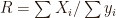
A ratio R can also be equally expressed as a measure of relative central tendency between the two variables, where n is the sample size:

The measure at the top of the ratio expression is known as the numerator and the measure at the bottom is the denominator.
Ratios enable evaluations of relationships in terms of relative comparisons. A ratio is a relative quantity between two amounts and measures the number of times that the numerator contains or is contained within the denominator.
The power of ratios
Ratios are powerful transformations because they enable standardised comparisons. They are numeraire-independent quantities, which means that they remove the effect of the original unit of measurement.
Consider the ratio of net income to assets (i.e. return on assets) of a large Australian mining company in 2010, as for example:
Net Income AU$ 10,000,000 as at 2010 / Assets AU$ 100,000,000 as at 2010
Now consider the same ratio of a much smaller French-based mining company in 2015, denominated in euro €:
Net Income € 1,000,000 as at 2015 / Assets € 5,000,000 as at 2015
It is not possible to cannot compare directly the Net Income or Assets of one company to the other because of different currencies, different points in time, as well as different sizes. That is to say, the Australian company employs AU$100 million assets to generate AU$1 million net income, whereas the French company only has € 5 million in assets.
However the resulting ratios of the two companies do not depend on scale, currency or time. The ratios are now expressed on a common unit of measurement which is the number of times that the numerator contains or is contained within the denominator.
Specifically, the Australian company’s return on assets is 0.1 which is not as good as the French company’s return on assets of 0.2.
Ratios can be found everywhere. Here are some more examples:
- Comparison of the profitability between two firms relative to their investment levels.
- Comparison of shareholders claims relative to the debt-holder claims.
- Comparison of indebtedness between countries relative to the market value of goods and services produced.
- Comparison of the tree girth in different forests relative to the tree length.
- Comparison of the growth in greenhouse emissions today relative to 100 years ago.
Note how every ratio involves a comparison that is a relative between two measures. The relative is the relation between the numerator and the denominator. The emphasis on comparison makes it clear it is best to judge a ratio on a comparative basis, using some sort of benchmark, threshold or rule of thumb.
Ratio bounds
Ratios may or may not have bounds, but understanding their range of variation is critical for interpretation.
Many ratios have bounds only on one end of the distribution, most typically on the left end because natural measurements are positively distributed. For example, the ratio of sales to operating assets is bounded at 0 on the left but is unbounded (i.e. is less than infinity) on the right. The zero bound on the left has a critical interpretation as it signifies a low turnover usage of the deployable assets.
Some ratios have unbounded distributions, extending to infinity in both the negative and positive side of the real line. For example, the popular price-to-earnings ratio (PE ratio) or the earnings yield (i.e. the inverse of the PE ratio) is such a case, because earnings can extend to a very large positive and a very large negative number.
In other cases, ratios may extend to very large numbers on technical grounds but such a bounds would be unrealistic, so we must consider theory to help us set some rule-of-thumb as expected bounds. For example, the human body-to-mass (BMI) index is defined as the mass (weight in kilos) over the squared height in centimetres. For the adult population, the World Health Organization gives interpretation guidelines for BMI ranging from 16 as ‘severe thinness’ to 40 as ‘obese class III’. Indeed, any values below 16 or above 40 would be unrealistic and could signify data entry errors.
Small value denominators
Numerators with the value of zero are meaningful as they turn the ratio into zero too, but denominators with zero values disable meaningful analysis as the ratio now becomes undefined, e.g. 4/0 = ∞.
Very small denominator values are also problematic because they yield very large ratio values, thus again possibly impairing useful interpretation relative to the rest of the density, e.g. 4/0.0001 = 40000.
Negative values
Negative values in ratios can lead to misleading inferences. We must pay particular care when the domain of the numerator and/or the denominator takes negative values because the division of a positive number with a negative number gives a negative number, and the division of a negative number with a negative number gives a positive number, e.g. 4/‐2 = ‐4/2 = ‐2 and ‐4/‐2 = 4/2 = 2.
When working with ratios involving such variables the analysis must be conditioned on these cases. A real example is the financial ratio of return on equity = Net Income / Equity. Both Net Income and Equity can take both negative and positive values, thus suggesting that ‐Earnings/Equity and Earnings/‐Equity would yield the same ratio. But these are two entirely different cases, the first describing company that is having a bad year and the second a company that is insolvent. Similarly, Earnings/Equity would give the same result as ‐Earnings/‐Equity.
Spurious ratio correlation
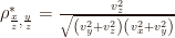
Another very bad practice is to talk about the correlation between two ratios that share a common denominator. Since Pearson (1896), we have been warned to be very careful of talking about correlations between ratios with a common denominator, because they artificially induce a portion of spurious correlation. y and x may be independent (have zero correlation), but when divided by a common denominator z, then the resulting ratios y/z and x/z are no longer independent. This holds for any y, x, z and even when z is independent to y and x. The ratio correlation between y/z and x/z is equal to:

where ρ is the Pearson product-moment correlation coefficients and v the coefficient of variation (standard deviation over the arithmetic mean). If y, x and z are independent to each other, then all ρ=0, which reduces the above equation to:
The difference between the two equations just above gives the approximate ‘true’ correlation that is directly attributed only to the linear association of the two numerators, y and x:

To demonstrate how pronounced is this effect, consider the following silly dataset with y the length of abalone, x the self-reported body-mass-index (BMI) of insurance customers, and z the price of whisky. This silly dataset is based on drawing random samples from real datas.
Let’s say that we are interested in the correlation between the length of abalone and BMI and, as expected, is very close to zero at –0.0074. This relation is shown in the left hand side graph just below:

Now divide the length of abalone and the BMI with the price of whisky, effectively creating the ratios y/z and x/z. The correlation between y/z and x/z is a whooping 0.9077, and the relation is shown in the right hand side graph. However, calculating the difference between the two formulas described above tell us that that the true portion of correlation is in fact a mere 0.003.
Ratios have inverses
You should always remember that ratios have inverses (or reciprocals). The ratio x/y may be just as informative, or even more so, to its inverse y/x.
The analysis on OECD top marginal tax rates demonstrates an example of such inverse ratio, whereby instead of talking about top tax thresholds relative to average earnings it is more intuitive to talk aboutaverage earnings relative to top tax threshold. In this way, the base value of 1 suggests that the top tax threshold in a country is set exactly equal to the income earnings by the average person or, in other words, the average person pays the top threshold.
Another example demonstrating the power of reciprocal ratios is the analysis on the miles-per-gallon illusion where it is shown that it far easier to form the correct decision in changing to more economic cars when thinking in terms of its inverse: gallon-per-miles.
Ratios of Normal distributions
I often stumble across the fatal mistake of dividing or multiplying a Normal distribution with another Normal distribution. To understand why you should never do that see the analysis on Ratios of Normal distributions.
Back to Recasting scales ⟵ ⟶ Continue to Data reduction
