Benford’s Law describes the expected frequency distribution of leading digits in positively distributed numerical series.
The law states that smaller digits are more likely to occur than larger digits. For example, it states that the leading digit of 1 appears about 30% of the time, whereas the leading digit of 9 appears less than 5% of the time.
Benford’s Law holds for variables that are positively distributed and grow in an exponential rate, such as volume of transactions, population, address numbers, births, and of course economic magnitudes such as sales, income and assets.
Benford’s Law can be applied to the first digit, second digit, third digit and further. However, for the first and second digit we expect a non-uniform
distribution, but as we move to the third digit and beyond the distribution
becomes near uniform.
The expected probability for the leading (first) digit being one of d = 1,…,9, in a series of numbers is determined by the following formula:
A more generalised formula for the expected probability that d = 1,…,9 appears as the digit n in a series of number, where n > 1, is as follows:

Graph objective
Benford’s Law is a useful auditing tool that is often applied in fraud detection for testing whether reporting does not natural expectations.
In this analysis, I will apply Benford’s Law to investigate whether the self-declaration of income in applications for life benefits insurance are as expected.
Data management
The data is commercially sensitive and cannot be shared. It contains about 6,000 applications of life benefits insurance. However, the Stata code that is provided at the end of this page can be easily adapted to any other related question and data.
The most important step in data management is to turn the numerical series into string and then use string functions to extract the first, second and third digits as separate variables.
Then, we apply logarithmic transformation to transform the proportion variable and the digits variable otherwise it would be impossible to see due to the exponential growth.
Visual implantations
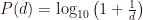
The series of expected probabilities is a growth-type of curve that can be naturally shown using a line implantation.
On this line, I encode point implantations to identify key numbers, including the first 9 leading digits (0, 1,… ,9) and the leading digits with 0 as the second digits (10, 20,…, 90).
In addition, I encode another series of line and point implantations that show the deviation of observed frequencies from the expected frequencies. The line encodes the extend of the deviation and the point serves as an anchor that enhance visual decoding, because decode lines alone is cumbersome.
Retinal variables
The colour retinal variable is employed to distinguish the expected frequency and the observed frequency, i.e. a categorical contrast. I choose to contrast dark shades of blue and red.
The shape retinal variable is used to distinguish the point implantations on the expected frequency line (hollow squares) and the observed frequency lines (filled in circles).
I also employ the size retinal variable to reduce the visual prominence of the points on the observed frequency line because they encode the same information as the lines.
Graph identification
Internal identification is achieved through a legend that is displayed on the top-right corner outside the plot region. The legend effectively identifies the colour retinal variable of the line implantations, and shows that anything in dark blue colour is related to expected frequencies, where anything in dark red colour is related to observed frequencies. So there is no need to disclose the point implantations because they are associated with these two colours.
Direct identification is an important step of the data graph. I directly identify next to the point implantations of the observed frequencies those cases that are extraordinarily larger than expected.
External identification includes a grand title, axes titles that explain the transformation in log scale, and detailed axes labels to enable table-look up.
Graph enhancement
An important graph enhancement step is the design of an appropriate axes grid, that would enable detailed table look-up for comparing and calculating the greater or lower than expected disclosures. I encode labels and grids only for the leading nine digits and all tens up to 100, otherwise it would be impossible to decode anything.
The aspect ratio is adjusted to be twice wide as tall because of the long curvilinear relation. This helps with encoding labels and decoding deviations from the expected frequency line.
Visual decoding/perception
Here is my proposed solution:
The observed frequencies that are larger than expected happen to be associated with the leading numbers of 10, 20, 30, 40, 50, 60 , 70, 80, 90 and the largest of all is 100, with 5.47% (5.9 – 0.43) more disclosures of income starting with 100 than expected. Naturally, as with many other disclosures, many people seem to like rounding up income to the nearest 10.
This may be because they do not remember exactly their income at the time of the life insurance application (not unlikely), but it could also be because they round up on purpose to hide their true income. The insurance company does not always verify income – it depends on the application.
Download the Stata code for reproducing this analysis: benford_income.do


