Graph objective
Life benefits insurance applications require the disclosure of personal data, including one’s height and weight. Regardless if the application is done face-to-face, perhaps through a financial adviser, or over the phone with an insurance telephone operator, or even online through an insurance aggregator, the applicant is asked to self-disclose the personal data. That is to say, there is no one who actually measures the exact height or weight. Knowing the actual height and weight is important because it forms the basis for calculating the body-to-mass (BMI) index, which is used to classify because as underweight, normal weight, overweight or obese.
One would expect that the adults would know their height with good accuracy, because for most males height will stop increasing at about 18, and for most females height growth halts at about 16. On the other hand, the self-disclosure of weight could be an approximation as weight changes regularly.
As it is impossible to know whether the disclosed height and/or weight are accurate, one way to evaluation the precision of this information is to look at the frequency of last digit for each number disclosed. It stands to reason to believe that nature would allow equal probability for weights and heights to end with the the value of 0,1,2,…,9. For example, observing more values ending with 0s or 5s would be a clear indication of rounding.
I must acknowledge that the investigation of this question is an original idea of Dr. Doron Samuell, a psychiatrist and insurance expert, who is also a close friend and research collaborator.
Data management
The data is sourced by a private insurance company; it it is commercially sensitive and cannot be shared. Note that the analysis here concerns only a a random sample of life insurance applications over several years.
The key data management step is the extract the last digit from each weight and height value. For example, for weight equal to 76 kilograms the last digit is 6, and for height 1.81 metres the last digit is 1.
The Stata code provided at the end of this page describes the steps for data management.
Visual implantations
I employ the point visual implantation in a scatter-plot to look at the cross-disclosure of the last digit for height and weight. Given the categorical values of 0,1,2,…,9 for each variable, the scatter plot will be a grid of 10 by 10, with overlapping values at each coordinate position.
Thus, if disclosure is accurate, then we expect that each position in this grid will contain roughly about 1% of observations. This statement is not entirely accurate, as Benford’s Law explains that we natural sequences of numbers have disproportionate distribution in the occurrence of digits (see also my analysis on Benford’s Law and income).
This disproportion is most evident in the leading (first) digits, where for example the leading number 1 is expect to occur about 30.1% of the time and the leading number 9 is expected to occur only 4.5% of the time. However, in this setting, where we are concerned with the investigation of the frequency in ending digits, notably at the second and third position, the distribution is roughly equivalent.
Retinal variables
Retinal variables are not instrumental to the construction of the proposed graph. I can get away with not using any differential retinal variables.
However, I employ a uniform colour retinal variable to encode all point implantations, and add a single point of another colour to those cross-categories that contain more than twice observations than the expected frequency.
Graph identification
The internal identification of the colour retinal variable is provided in a legend that identifies densities that indicate cases of extraordinarily large frequencies.
External identification includes a title describing the key question, axes titles describing the variables and their unit of measurement, and the axes labels that show the cross-tabulation of the last digits.
I also directly identify the observed percentages of those frequencies that represent cases with more than twice than the expected frequency of 1%.
Graph enhancement
The key to the construction of the proposed graph is a graph enhancement tool, specifically that of jittering.
Jittering adds a random portion of variation to each value, that moves its location to any direction around the original coordinate. You can think about jittering as ‘shaking’ a density to reveal the overlapping coordinates. In this way, we can get an idea of the extend of each density in a fixed location.
Visual decoding/perception
Here is my proposed solution:
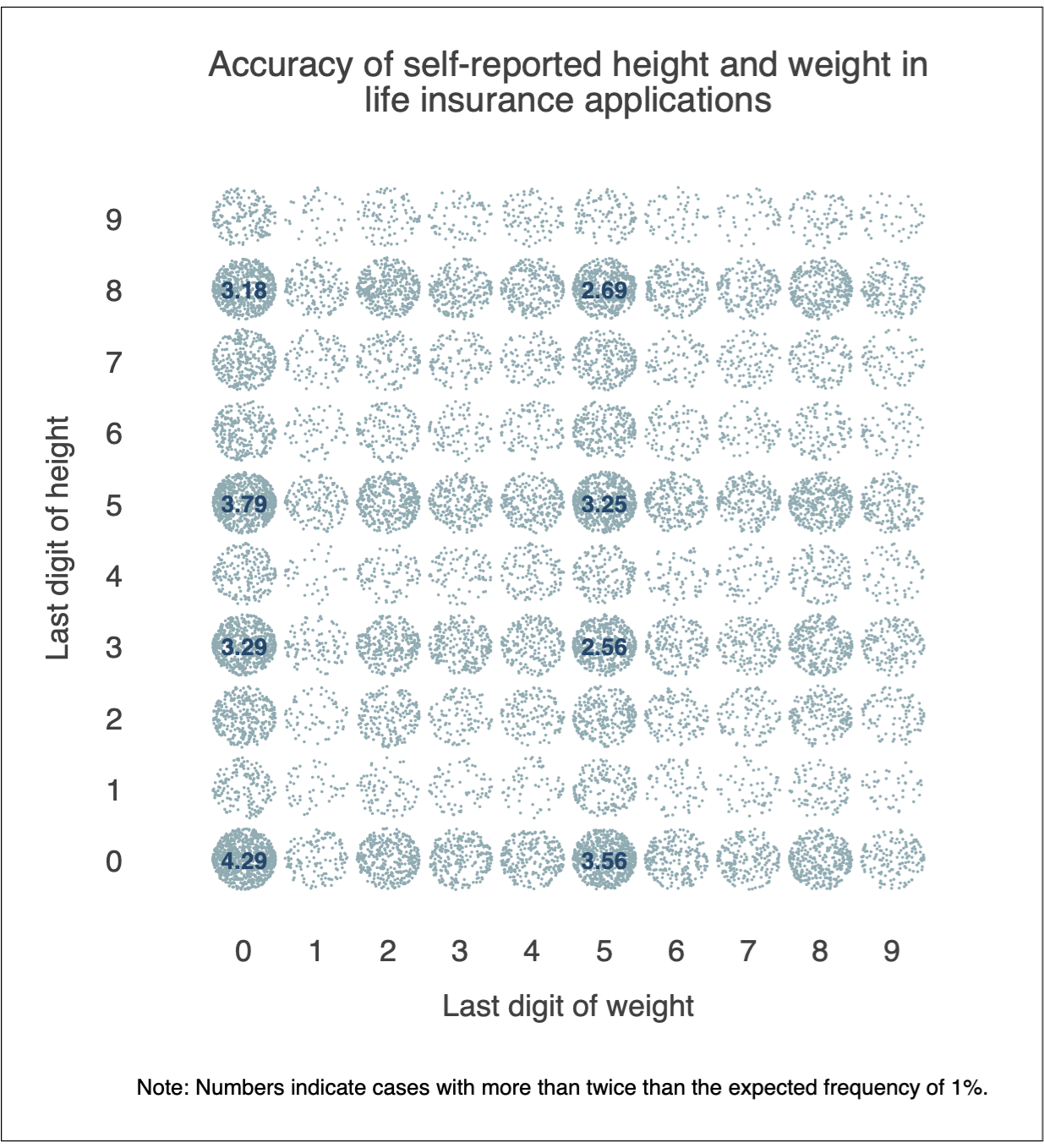
It is clear that most people like to round their weight and height to the nearest 0 or 5, so it is unsurprisingly to see that the most frequent cross-category is (0,0). This is a natural thing to do as we train from early age to count numbers on our fingers, and finally progress to using the decimal numeral system. This is especially true in weight given the approximate calculation.
It is surprising to see, however, the high frequency of 8s and 3s in height. It is beyond my understanding why there are so many heights ending with an 8 or a 3. If someone knows then please let me know.
At the same time, the least frequent disclosure is the digit of 9, in both heights and weights. One could argue that this question should be best investigated using Benford’s Law, that states that the occurrence of 9 as a second digit mostly in weight is about 8.5% likely and as a third digit in height is about 9.8% as likely. Even so, this does not explain the excessively low disclosures of 9s seen above.
As an example, you can have a look at my analysis on Benford’s law and income.
Download the Stata code for reproducing this analysis: height_weight.do


